Classifying street networks of 58 cities
Is a city a grid, organically grown, or shaped by hills? I downloaded the street networks of 58 cities worldwide from OpenStreetMap, computed four structural metrics per network, and grouped the cities by type, using only the street graph and no information about location.
01 / Overview
Motivation
Street networks encode a city's history and terrain. Karlsruhe was planned as a fan of streets radiating from its palace, Manhattan as a strict rectangular grid, while Bilbao follows the valleys between the surrounding hills. Can these structural types be recovered from the street graph alone?
I computed four metrics per network and used them to group all 58 cities, based purely on structure, without any knowledge of geographic origin.
02 / Data
58 street networks from OpenStreetMap
For each city, the central 50 km² were retrieved with OSMnx; Manhattan was included at its full area of 59.1 km². The sample covers Europe, North and South America, Asia, and Australia.
- Nodes: intersections and dead ends
- Edges: street segments between nodes, stored as polylines
- 30+ built-in OSMnx statistics per network, plus four metrics I computed myself
03 / Metric 1: Grid Perfectness
Street orientation Θ
Following Geoff Boeing's approach, the compass bearing of every street segment (and its reverse) is sorted into 10° bins. Opposite bins are paired to capture the symmetry of a grid, and the Shannon entropy of the resulting distribution is converted into a grid-perfectness score Θ between 0 and 1, where 1 is a perfect grid.
Three grid types
- Group A (Θ < 0.15): 47 cities with organic networks. Toulouse has the lowest value (Θ = 0.002), an almost uniform distribution of directions.
- Group B (0.15–0.45): 6 cities with partial grids, including Barcelona and San Francisco.
- Group C (Θ > 0.45): 5 cities with near-perfect grids: Portland (0.778), Manhattan (0.651), Montreal, Toronto, and Osaka.
Examples: orientation plots by group
Browse the three grid types
Group A — Θ < 0.15 — Organic
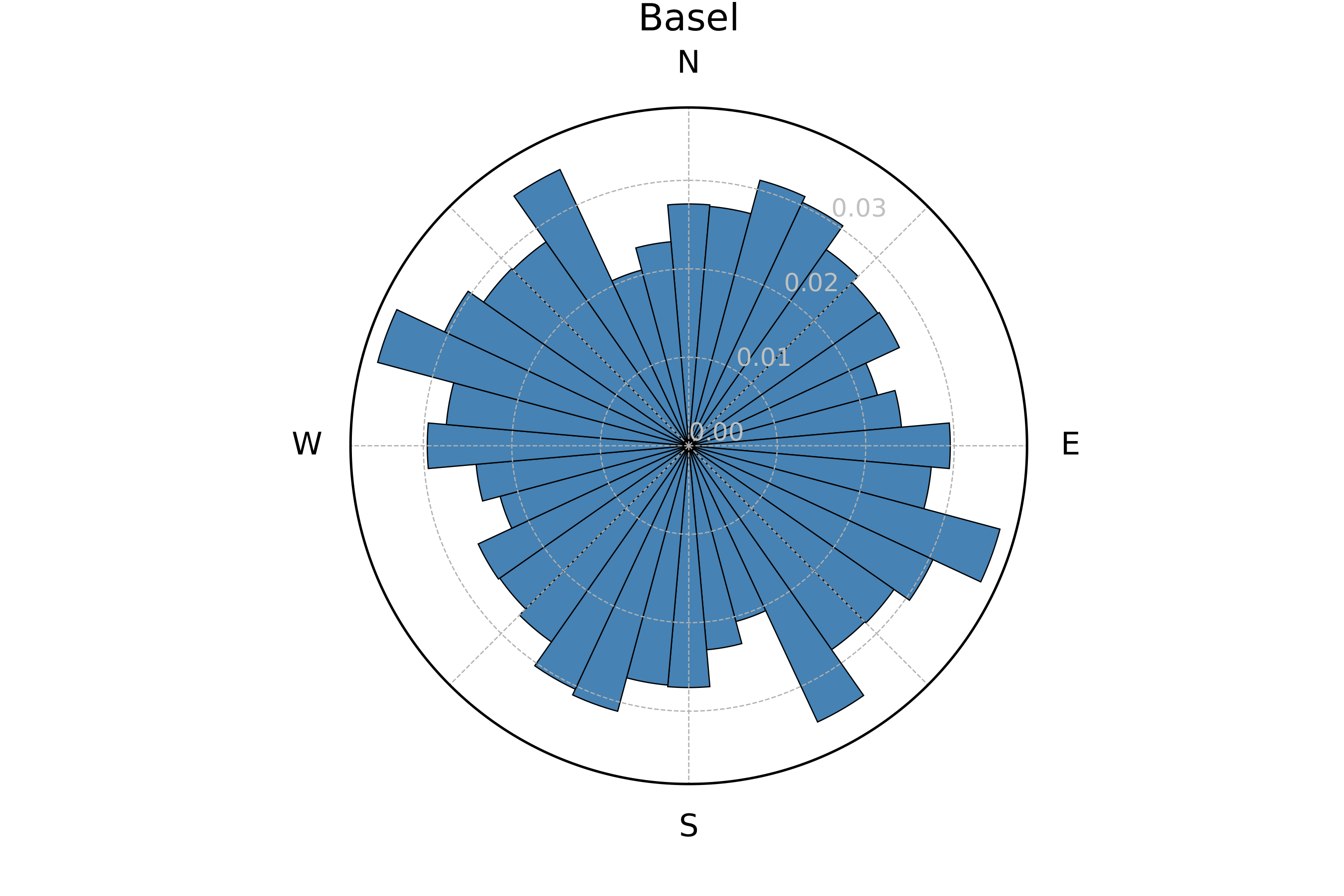
Basel — Θ = 0.008
Group B — 0.15–0.45 — Partial grid
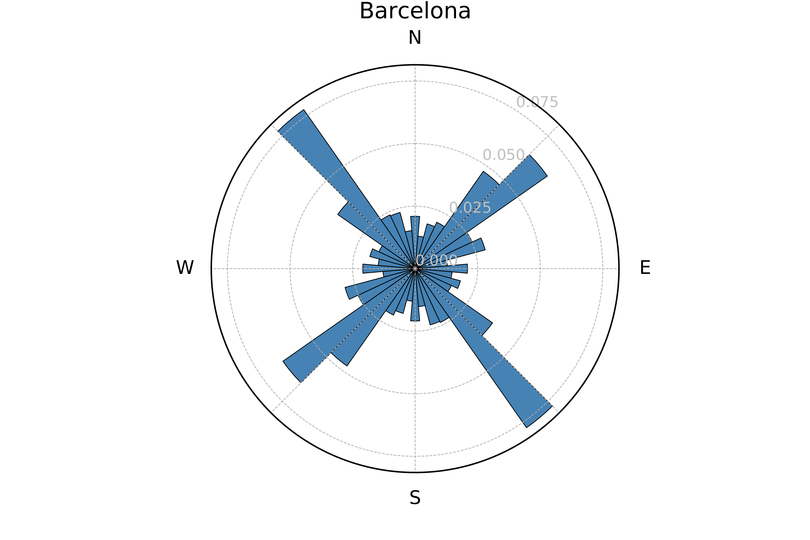
Barcelona — Θ = 0.160
Group C — Θ > 0.45 — Perfect grid
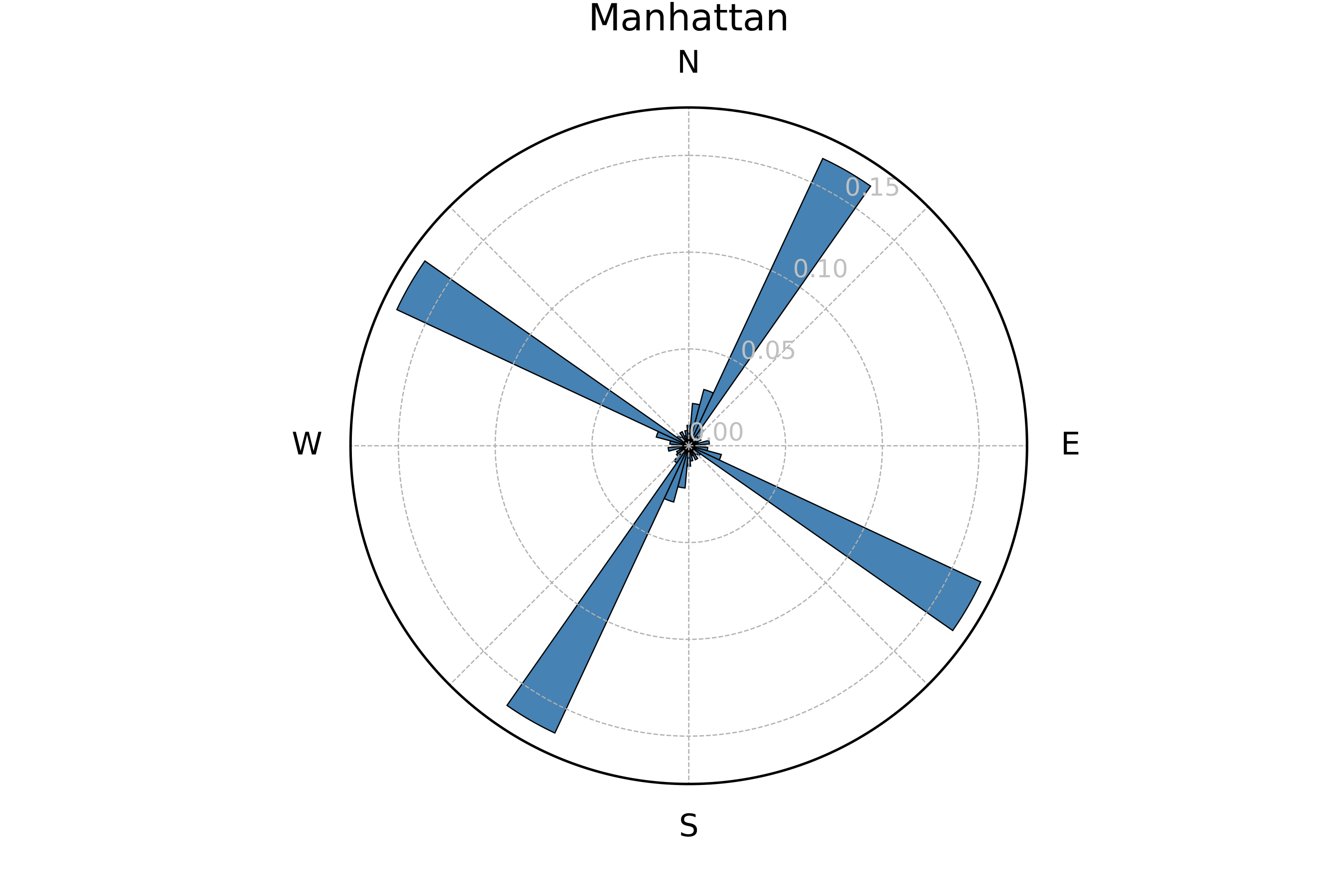
Manhattan — Θ = 0.651
04 / Metric 2: Empty Space
Void points ε
Large areas without streets, such as forests, lakes, or hills, force long detours. To measure this, a 60 × 60 grid of probe points (about 125 m apart) is laid over each network. A probe counts as an ε-void if no street lies within 250 m. A city without any streets would have 3,600 voids.
- Katowice (ε = 798): the maximum, shaped by forests and parks
- Tokyo (ε = 0): no gap large enough anywhere
- Strong negative correlation with node count: denser networks have fewer voids
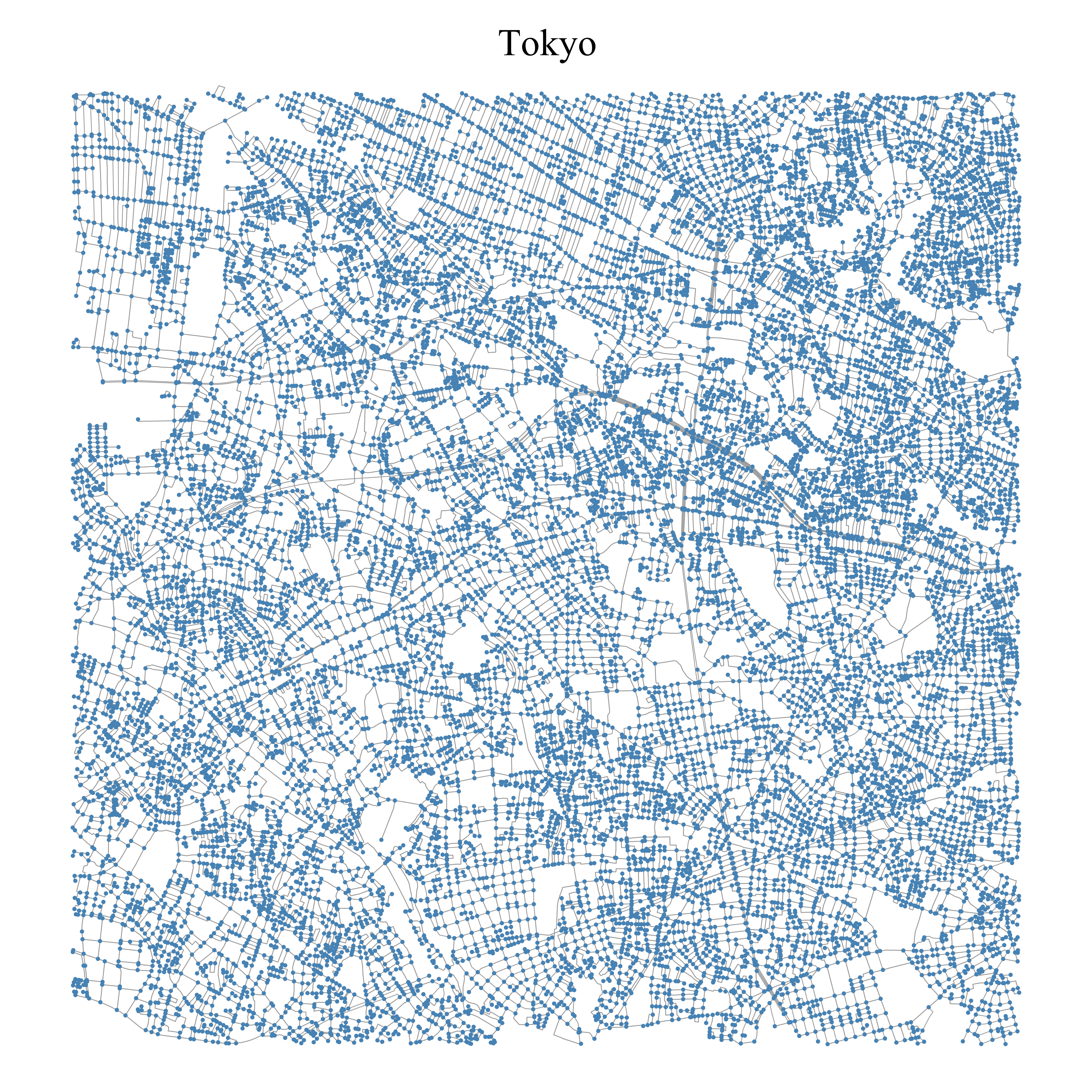
Tokyo: ε = 0
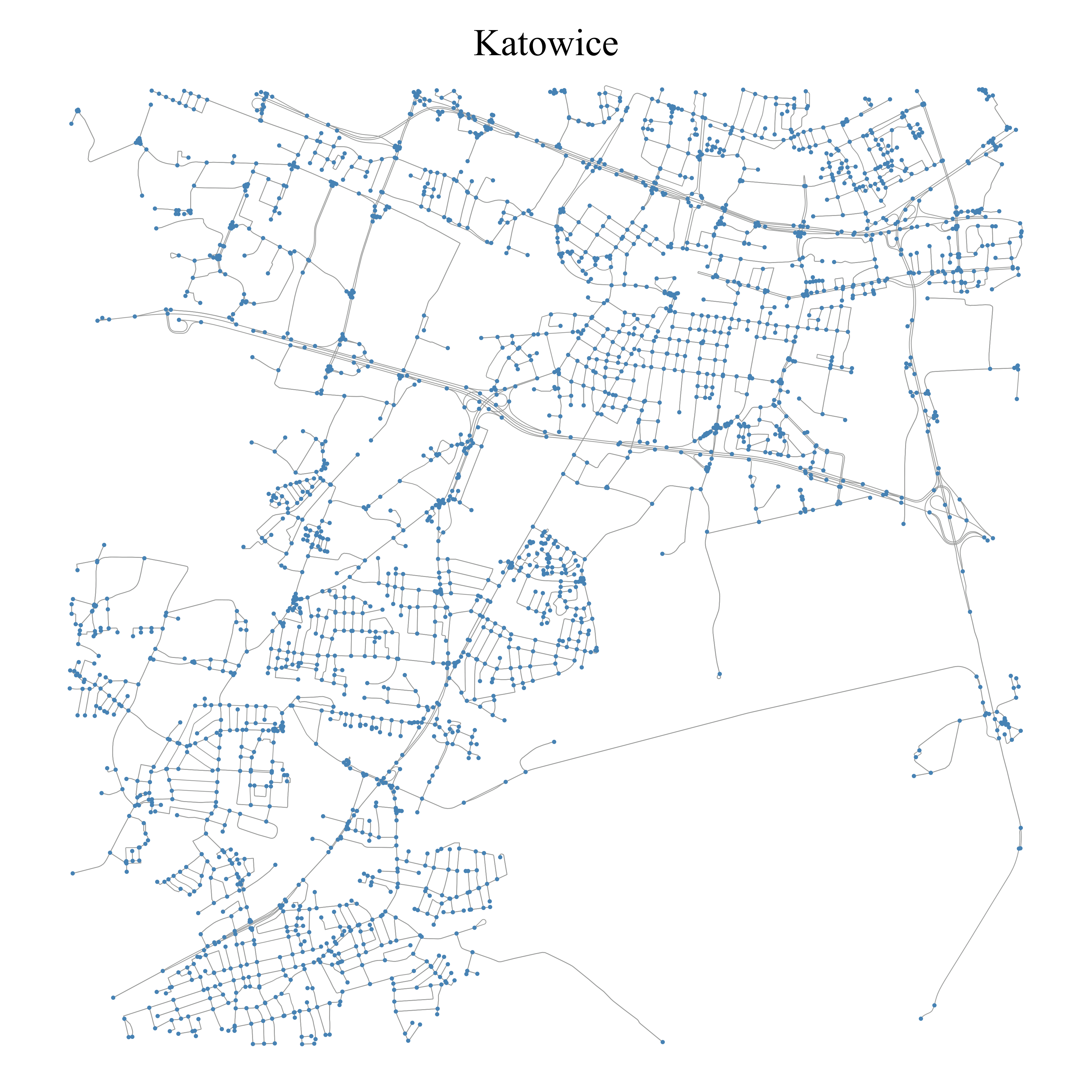
Katowice: ε = 798
05 / Metric 3: Edge Curvature
Mean geometry index
OSMnx stores curved streets as polylines. The geometry index of a street segment counts how many straight lines are needed to draw it: a straight road has index 1, a winding mountain road 20 or more. The mean over all segments characterizes the network.
- α (index < 3): 15 cities, e.g. Nagoya and Tokyo, with dense, flat, short segments
- β (3–5): 37 cities, including most European cities
- γ (index > 5): 6 cities: Linz, Helsinki, Karlsruhe, Saarbrücken, Bilbao, and Geneva
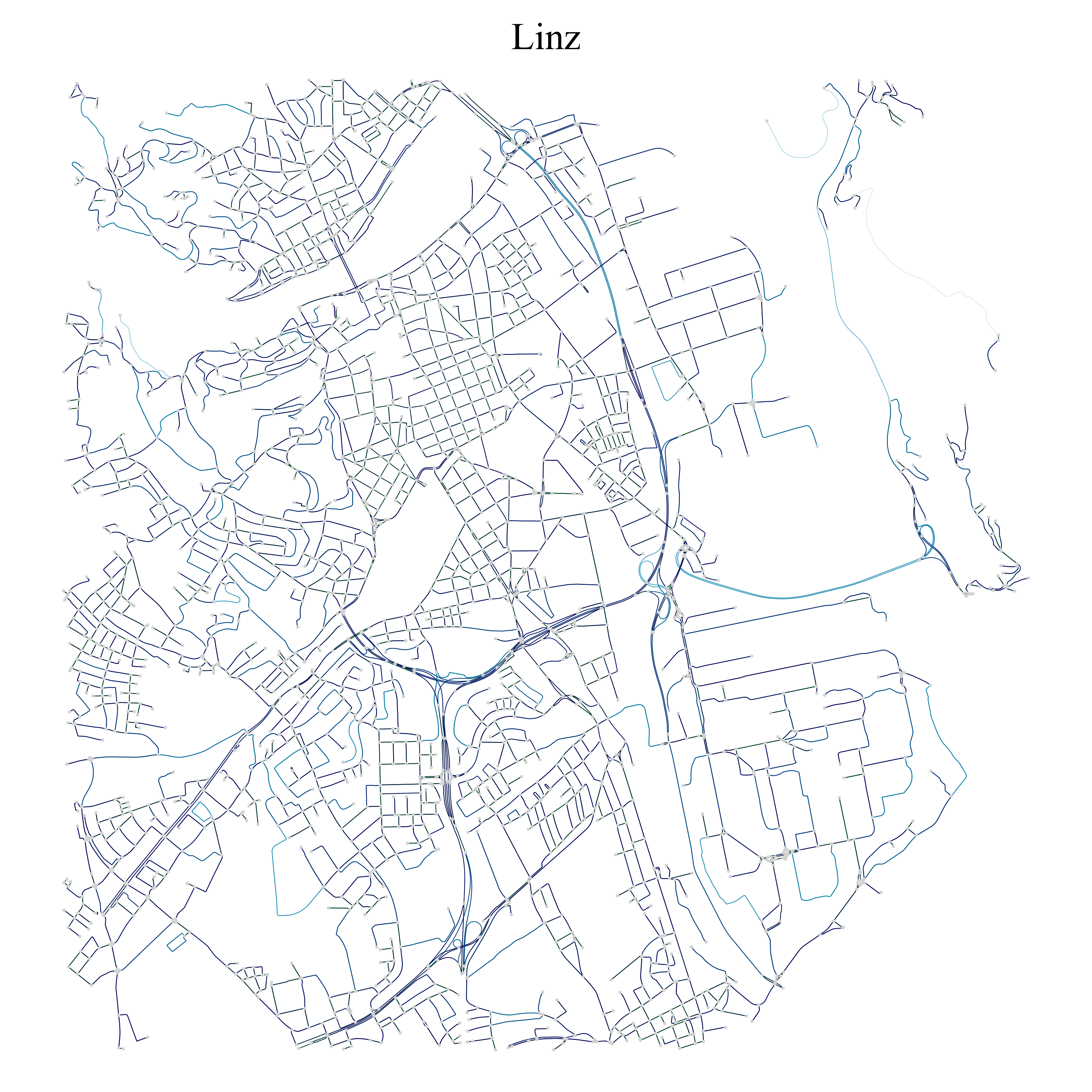
Linz: 8.282
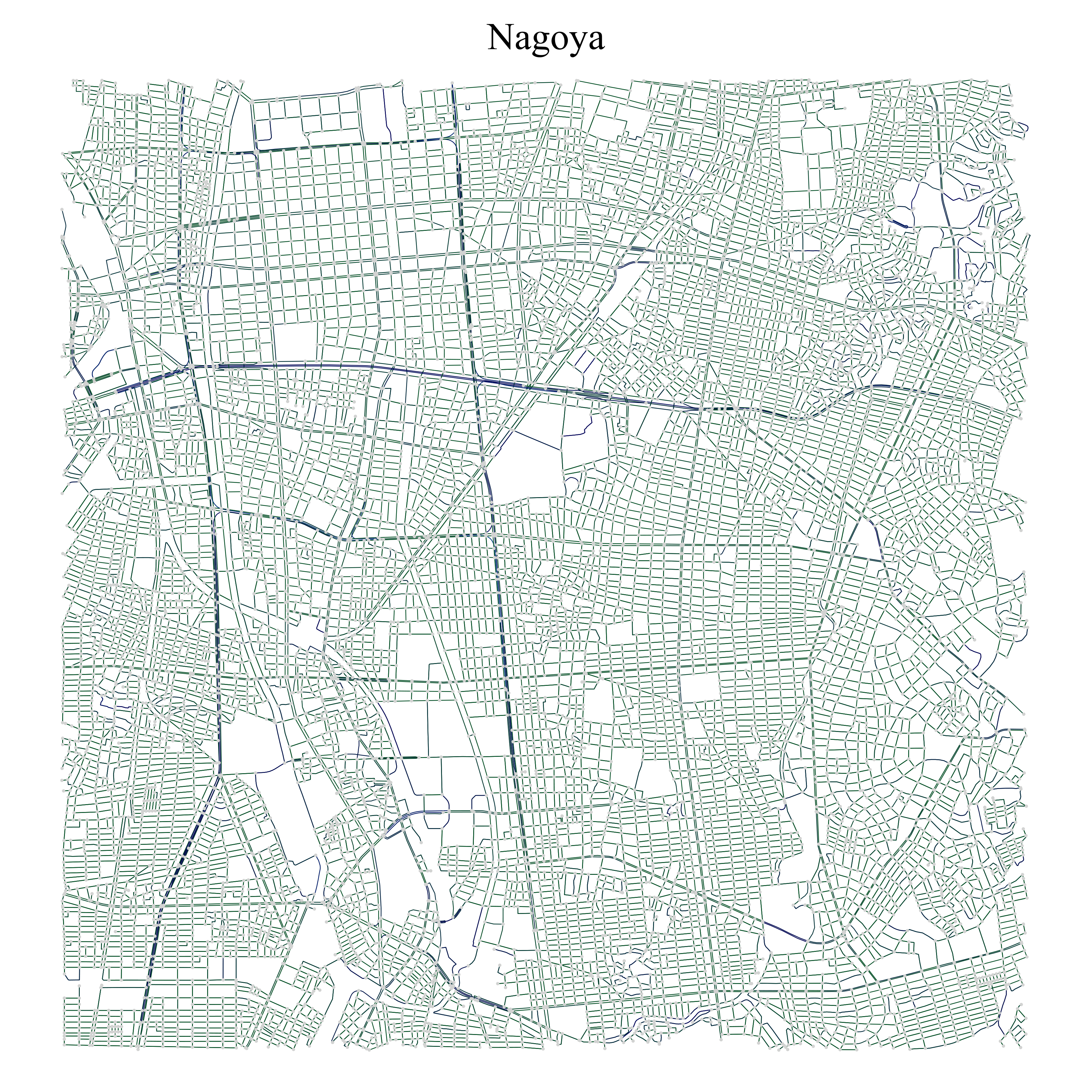
Nagoya: 1.405
06 / Metric 4: Connectivity
Optimal number of clusters
How many hubs does a city need so that every intersection is close to one? The optimal number of clusters is the smallest m for which the mean shortest-path distance from each node to its nearest cluster center falls below 2,000 m. Centers are seeded with k-means on the coordinates, snapped to the nearest real intersection, and shortest paths are computed with NetworkX.
- Seoul: 2 clusters, a flat and well-connected network
- Bilbao: 6 clusters, as hills and valleys force long detours
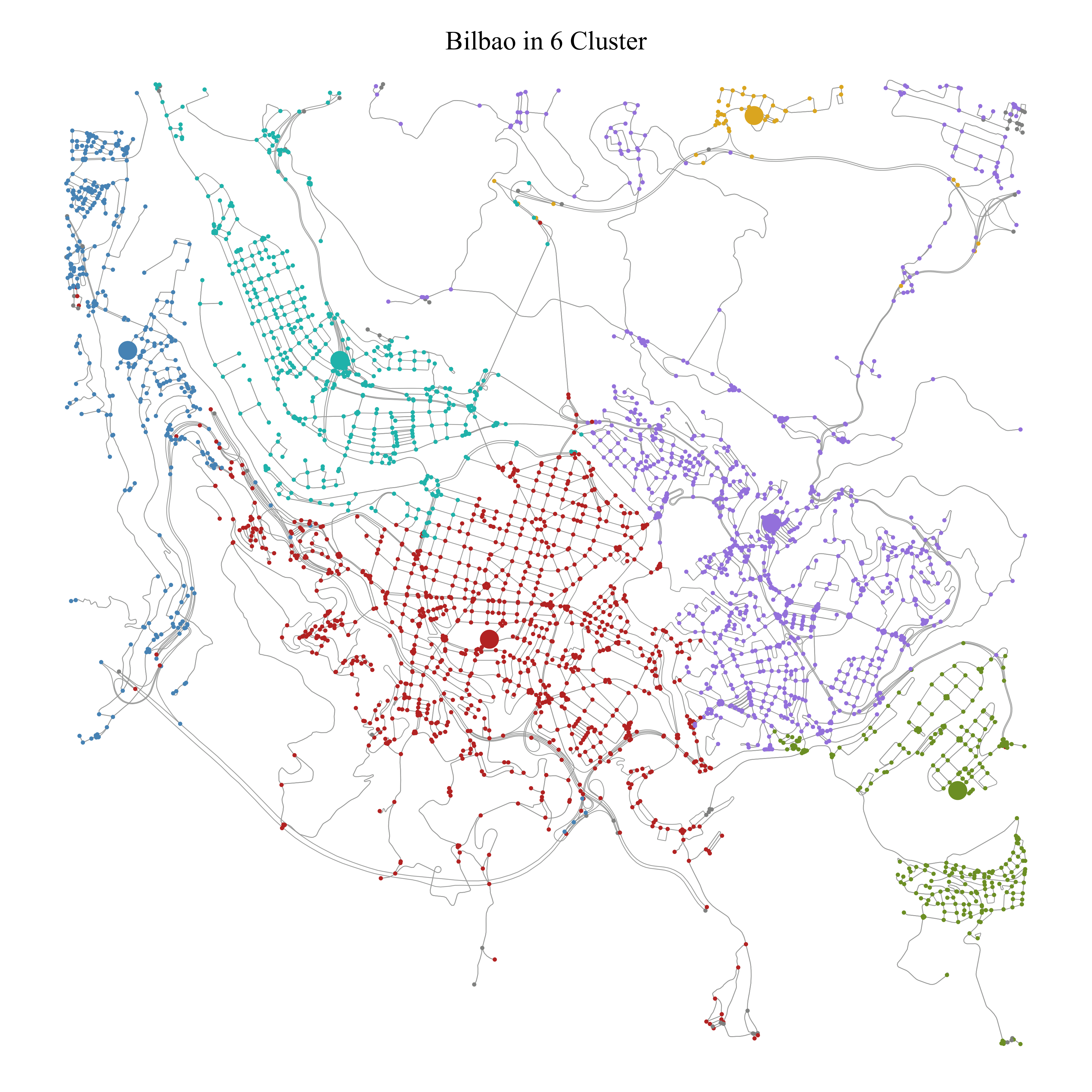
Bilbao: 6 clusters
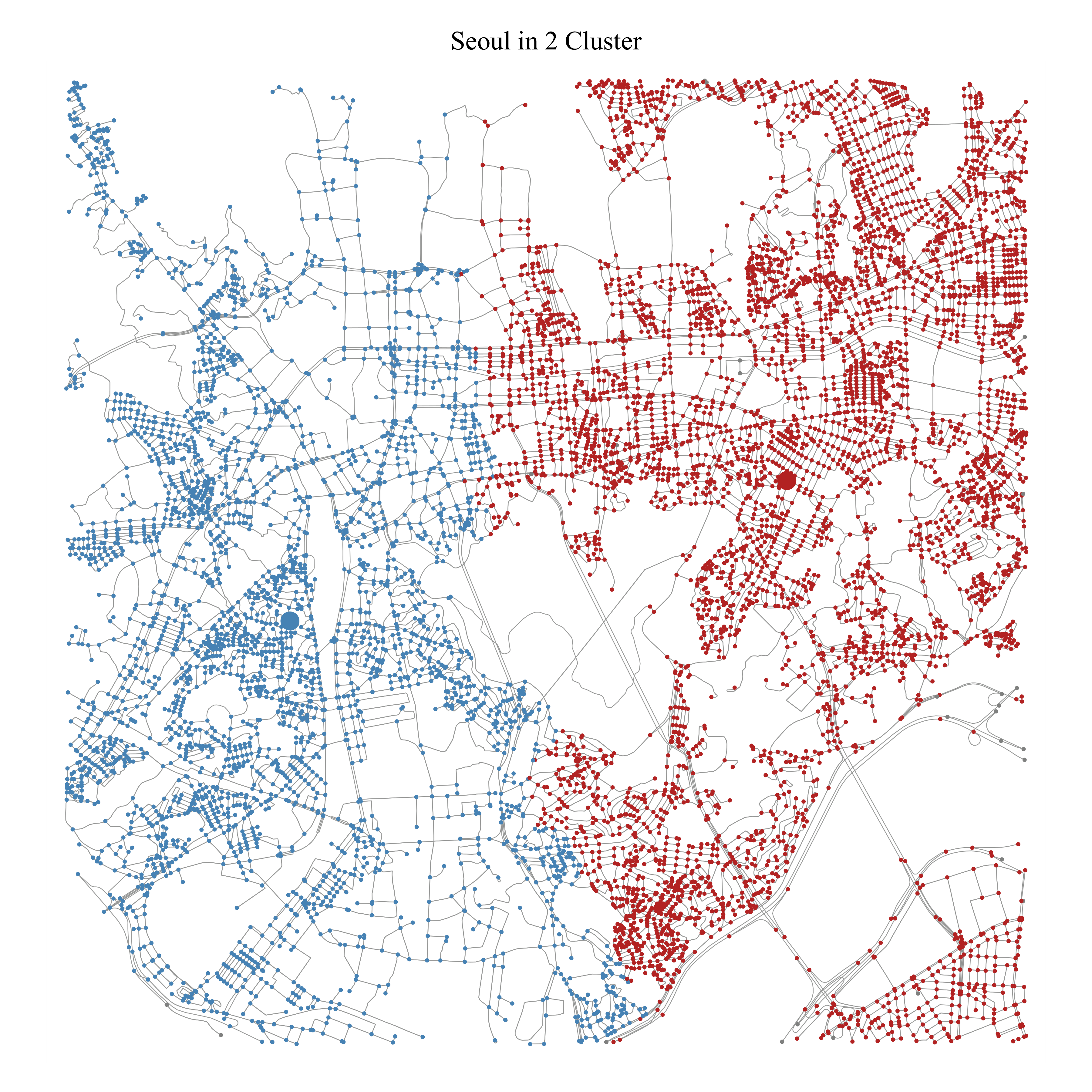
Seoul: 2 clusters
07 / Results
City classifications
The metrics correlate moderately, but each captures a distinct aspect of the network. Together they tell a consistent story: flat, planned cities have a high Θ, few voids, and a low geometry index; hilly, organically grown cities show the opposite.
- Portland: highest grid perfectness (Θ = 0.778)
- Katowice: most empty space (ε = 798)
- Linz: most curved streets (index 8.282)
- Seoul: best connected (2 clusters)
- Bilbao: most fragmented by terrain (6 clusters)
Selected cities: all four metrics
| City | Θ | Group | ε-voids | Geom. | Clusters |
|---|---|---|---|---|---|
| Toulouse | 0.002 | A | 85 | 4.051 | 4 |
| Barcelona | 0.160 | B | 228 | 3.439 | 4 |
| San Francisco | 0.307 | B | 6 | 3.974 | 3 |
| Osaka | 0.519 | C | 16 | 1.480 | 3 |
| Manhattan | 0.651 | C | 0 | 3.118 | 4 |
| Portland | 0.778 | C | 77 | 2.871 | 3 |
| Katowice | 0.079 | A | 798 | 4.606 | 4 |
| Linz | 0.047 | A | 397 | 8.282 | 3 |
| Seoul | 0.032 | A | 150 | 2.458 | 2 |
| Tokyo | 0.053 | A | 0 | 1.872 | 3 |
08 / Conclusion
Structure reveals city type
The four metrics separate street networks by structure alone, without reference to geography. Their combination yields consistent conclusions about terrain, planning history, and connectivity that match known characteristics of the cities.
The approach could support cross-city comparisons, for example as a basis for benchmarking infrastructure.
Limitations and next steps
What could be improved
The analysis uses central 50 km² cutouts; Boeing's work suggests these approximate whole-network statistics well.
- More cities: 58 networks is a small sample; more cities would sharpen the group boundaries.
- Elevation data: would make the terrain conclusions quantitative rather than interpretive.
- District borders: administrative boundaries could enrich the connectivity analysis.
- Change over time: street networks evolve; a temporal analysis is an open extension.